

How To Draw Q-q Plot Using Python
Python and Matplotlib tin be used to create static 2D plots. But it Matplotlib tin can also be used to create dynamic auto-updating animated plots. In this postal service, yous learn how to create a live auto-updating animated plot using Python and Matplotlib.
Tabular array of contents:
- Pre-requisits
- Gear up up a Python virtual environment
- Install Python packages
- Create a static line plot
- Import packages
- Create an animated line plot
- Build a live plot based on user input
- Build a alive plot using data from the web
- Build a live plot using data from a sensor
- Hardware Hookup
- Arduino Code
- Python Code
- Summary
- Support
Pre-requisits
To follow along with this tutorial, a couple of pre-requisites demand to exist in place:
- Python needs to be installed on your reckoner. I recommend installing the Anaconda Distribution of Python.
- You are running a version of Python 3.6 or above. Python version three.vii or iii.eight are more up-to-date and recommended.
- Yous know how to open the Anaconda Prompt on Windows10 or know how to open a terminal on MacOS or Linux.
- You have a general idea of what Python packages are and accept installed a Python package before using conda or pip.
- Yous know how to create a text file in an editor or an IDE (integrated development surround) such every bit Visual Studio Code, PyCharm, Sublime Text, vim, emacs, etc. I will be using Visual Studio Code (also chosen VS Lawmaking) in this post, but any regular code editor volition work.
- You lot know how to run a Python program (execute a .py file) using a final prompt, like the Anaconda Prompt, or know how to run a Python program using your IDE.
- You have a general understanding of how files are organized on your calculator into directories and sub-directories.
- Yous have some familiarity with navigating through directories and files using a terminal or the Anaconda Prompt with commands like
cd,cd ..,dirorls, andmdkir.
Now that the pre-requisites are out of the way, let'due south commencement coding!
Set upwardly a Python virtual environment
To offset the coding process, we volition ready a new Python virtual environment.
Real Python has a good introduction to virtual environments and why to use them.
I recommend undergraduate engineers utilise the Anaconda distribution of Python which comes with the Anaconda Prompt. You tin can create a new virtual environment by opening the Anaconda Prompt and typing:
Using the Anaconda Prompt:
> mkdir live_plot > cd live_plot > conda create -y -n live_plot python=3.7 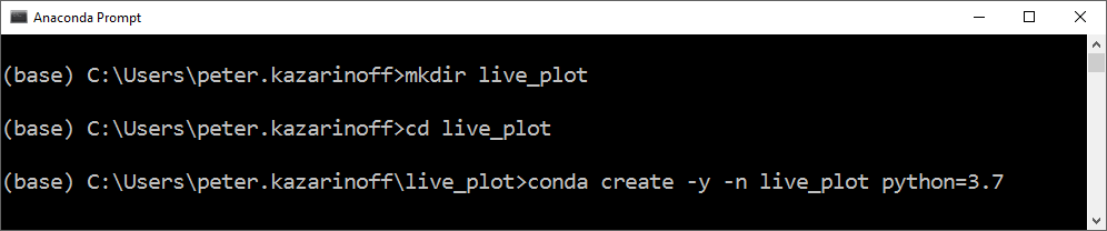
Alternatively, on MacOS or Linux, a virtual surroundings tin can exist set up up with a terminal prompt and pip (the Python packet manager).
Using a terminal on MacOS or Linux:
$ mkdir live_plot $ cd live_plot $ python3 -m venv venv Install Python packages
Now that we have a new clean virtual environs with Python iii installed, nosotros need to install the necessary packages that nosotros'll use to create our plots.
Using the Anaconda Prompt, actuate the live_plot virtual environment and utilize conda to install the post-obit Python packages. Ensure the virtual surround you lot created to a higher place is activate when the packages are installed.
> conda activate live_plot (live_plot)> conda install -y matplotlib requests pyserial 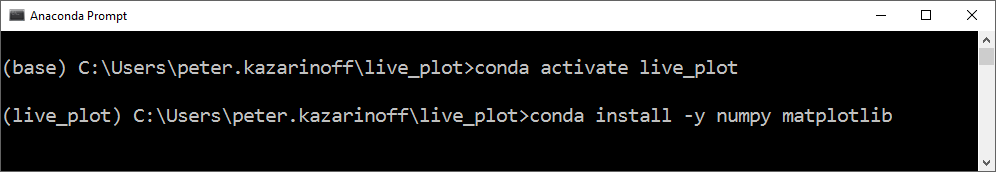
Alternatively, if you are using MacOS or Linux, the packages can be installed with a terminal pip:
$ source venv/bin/activate (venv) $ pip install matplotlib (venv) $ pip install requests (venv) $ pip install pyserial Create a static line plot
Before we create a live blithe motorcar-updating plot, let's outset create simpler static, not-moving line plot. Our alive plots will look a lot like this starting time static plot, except in the live plot, the line on the plot will move. Coding a simpler plot outset gives united states some do and a structure to build upon when we create the more complex live plots.
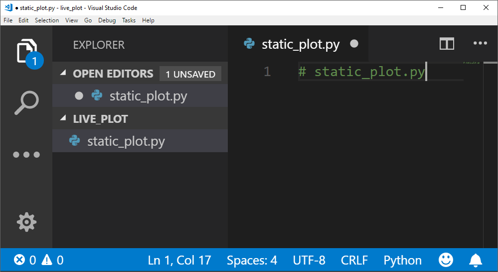
Open a text editor or IDE (I like to employ VS Code) and create a new Python file called static_plot.py
Import packages
Let's start our static_plot.py script by importing the packages nosotros'll use later in the script. Matplotlib's pyplot module is imported using the standard allonym plt.
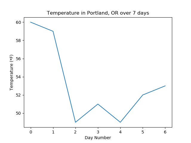
# static_plot.py # import necessary packages import matplotlib.pyplot as plt We need some data to plot. For this first static plot, nosotros'll plot the temperature in Portland, OR in degrees Fahrenheit over seven days. We'll salvage the temperatures in a Python list called data_lst.
# data data_lst = [ 60 , 59 , 49 , 51 , 49 , 52 , 53 ] Side by side, we'll create a figure object fig and an axis object ax using Matplotlib's plt.subplots() method.
# create the figure and centrality objects fig , ax = plt . subplots () Now we tin plot the temperature data on the axis object ax and customize the plot. Let's include plot championship and axis labels.
# plot the information and customize ax . plot ( data_lst ) ax . set_xlabel ( 'Day Number' ) ax . set_ylabel ( 'Temperature (*F)' ) ax . set_title ( 'Temperature in Portland, OR over 7 days' ) Finally, we tin can bear witness and save the plot. Make sure that the fig.savefig() line is before the plt.prove() line.
# save and bear witness the plot fig . savefig ( 'static_plot.png' ) plt . show () That'due south it for this first script. Pretty elementary correct?
Run the static_plot.py script using the Anaconda Prompt of a terminal. Ensure the virtual environment (live_plot) is active when the script is run.
(live_plot)> python static_plot.py 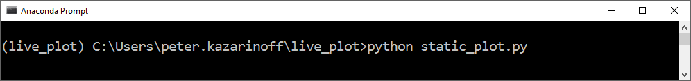
The plot should look something like the prototype below:
The complete script is beneath:
# static_plot.py # import necessary packages import matplotlib.pyplot as plt # data data_lst = [ 60 , 59 , 49 , 51 , 49 , 52 , 53 ] # create the figure and centrality objects fig , ax = plt . subplots () # plot the data and customize ax . plot ( data_lst ) ax . set_xlabel ( 'Day Number' ) ax . set_ylabel ( 'Temperature (*F)' ) ax . set_title ( 'Temperature in Portland, OR over 7 days' ) # save and show the plot fig . savefig ( 'static_plot.png' ) plt . show () Next, we'll build an animated line plot with Matplotlib.
Create an animated line plot
The previous plot nosotros just built was a static line plot. We are going to build upon that static line plot and create an blithe line plot. The data for the animated line plot volition be generated randomly using Python's randint() function from the random module in the Standard Library. Python's randint() function accepts a lower limit and upper limit. We will set a lower limit of ane and an upper limit of 9. The script to build the animated line plot starts almost the same manner as our simple line plot, the departure is that we demand to import Matplotlib's FuncAnimation class from the matplotlib.animation library. The FuncAnimation class will be used to create the blithe plot.
# animated_line_plot.py from random import randint import matplotlib.pyplot as plt from matplotlib.animation import FuncAnimation # create empty lists for the ten and y information 10 = [] y = [] # create the figure and axes objects fig , ax = plt . subplots () In our starting time static line plot, we started the plot at this betoken, merely for the animated line plot, we need to build the plot in a function . At a minimum, the office that builds the plot needs to have one argument that corresponds to the frame number in the blitheness. This frame number argument tin exist given a simple parameter similar i. That parameter does not have to be used in the function that draws the plot. It just has to exist included in the function definition. Note the line ax.clear() in the middle of the role. This line clears the effigy window so that the next frame of the animation can exist drawn. ax.clear() needs to be included before the data is plotted with the ax.plot() method. Besides, note that plt.show() is not function of the role. plt.bear witness() will be called exterior the function at the end of the script.
# office that draws each frame of the blitheness def animate ( i ): pt = randint ( 1 , 9 ) # take hold of a random integer to exist the next y-value in the animation 10 . append ( i ) y . append ( pt ) ax . articulate () ax . plot ( x , y ) ax . set_xlim ([ 0 , 20 ]) ax . set_ylim ([ 0 , 10 ]) OK- our animate() part is divers, at present we need to call the animation. Matplotlib's FuncAnimation class can accept several input arguments. At a minimum, we demand to pass in the figure object fig, and our animation role that draws the plot animate to the FuncAnimation class. Nosotros'll also add together a frames= keyword argument that sets many times the plot is re-drawn significant how many times the animation function is called. interval=500 specifies the fourth dimension between frames (time between animate() function calls) in milliseconds. interval=500 ways 500 milliseconds between each frame, which is one-half a 2nd. echo=False ways that after all the frames are fatigued, the animation will not repeat. Notation how the plt.show() line is called after the FuncAnimation line.
# run the animation ani = FuncAnimation ( fig , animate , frames = twenty , interval = 500 , repeat = False ) plt . evidence () You tin run the animated_line_plot.py script using the Anaconda Prompt or a final.
(live_plot)> animated_line_plot.py An example of the plot blithe line plot produced is beneath.
Side by side, we'll build a alive auto-updating plot based on user input.
Build a live plot based on user input
Create a new Python file called live_plot_user_input.py using a code editor or IDE.
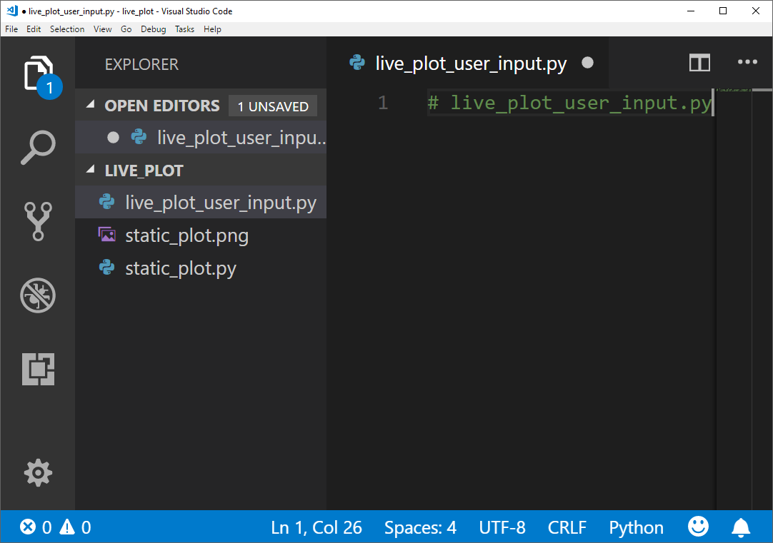
In the file live_plot_user_input.py, add the same imports nosotros used in our previous plot: Matplotlib's pyplot library is imported as plt and Matplotlib's FuncAnimation class is imported from the matplotlib.animation library. Like the previous plot, we'll use the FuncAnimation class to build our live auto-updating plot and create an animation() function to draw the plot.
# live_plot_user_input.py # import necessary packages import matplotlib.pyplot as plt from matplotlib.animation import FuncAnimation Side by side, we'll pre-populate a list called information with a couple of information points. This will gives our plot a couple of points to start off with. When our script runs, we'll include functionality to add more points.
# initial data data = [ 3 , half dozen , 2 , 1 , 8 ] # create figure and axes objects fig , ax = plt . subplots () Now we'll build an breathing() office that volition read in values from a text file and plot them with Matplotlib. Note the line ax.articulate(). This line of code clears the current centrality so that the plot can exist redrawn. The line ax.plot(information[-5:]) pulls the last 5 data points out of the list data and plots them.
# animation function def breathing ( i ): with open up ( 'information.txt' , 'r' ) as f : for line in f : information . append ( int ( line . strip ())) ax . clear () ax . plot ( data [ - five :]) # plot the last 5 data points The last section of code in the live_plot_user_input.py script calls the FuncAnimation class. When we instantiate an instance of this class, we pass in a couple of arguments:
-
fig- the figure object we created with theplt.subplots()method -
animate- the office we wrote higher up that pulls lines out of adata.txtfile and plots 5 points at a time. -
interval=1000- the time interval in milliseconds (1000 milliseconds = 1 second) between frames or betweenanimate()function calls.
# call the animation ani = FuncAnimation ( fig , animate , interval = m ) # evidence the plot plt . show () Before you run the script, create a new file in the live_plot directory aslope our live_plot_user_input.py script chosen information.txt. Inside the file add together a couple of numbers, each number on one line.
Save data.txt and leave the file open. This is the file that nosotros will add numbers to and watch our live plot update.
Save live_plot_user_input.py and run information technology. You should meet a plot popular up.
At present add a number to the bottom of the data.txt on a new line. Relieve data.txt. The plot should update with a new data signal. I added the number 16 to data.txt and saw the line on the plot go upwards. Add another number at the end of data.txt. Save information.txt and sentinel the plot update.
Great! We built a live-updating plot based on user input! Next, let's build a alive automobile-updating plot using data pulled from the web.
Build a live plot using information from the web
The third plot we are going to build is a plot that pulls data from the spider web. The basic construction of the script is the same as the terminal two animated plots. Nosotros need to create figure and axis objects, write an animation function and create the blitheness with FuncAnimation.
https://qrng.anu.edu.au/API/api-demo.php
The website notes:
This website offers truthful random numbers to anyone on the net. The random numbers are generated in real-time in our lab by measuring the quantum fluctuations of the vacuum.
Having true random numbers for an animated plot isn't absolutely necessary. The reason I picked this web API is that the random numbers can be polled every second, and since you lot tin specify an viii-bit integer, the random numbers accept a fixed range between 0 and 255.
The code beneath calls the spider web API for one 8-bit random integer. A little function converts the web API'due south JSON response into a float. The raw JSON that comes back from the API looks similar below:
{ "type" : "uint8" , "length" : 1 , "data" :[ 53 ], "success" : true } In one case the JSON is converted to a Python lexicon, we can pull the random number out (in this case 53) with the post-obit Python code.
The entire script is beneath.
# plot_web_api_realtime.py """ A live machine-updating plot of random numbers pulled from a web API """ import time import datetime every bit dt import requests import matplotlib.pyplot every bit plt import matplotlib.animation every bit animation url = "https://qrng.anu.edu.au/API/jsonI.php?length=one&type=uint8" # function to pull out a bladder from the requests response object def pull_float ( response ): jsonr = response . json () strr = jsonr [ "data" ][ 0 ] if strr : fltr = round ( bladder ( strr ), 2 ) return fltr else : return None # Create effigy for plotting fig , ax = plt . subplots () xs = [] ys = [] def animate ( i , xs : listing , ys : list ): # grab the data from thingspeak.com response = requests . become ( url ) flt = pull_float ( response ) # Add together x and y to lists xs . append ( dt . datetime . now () . strftime ( '%H:%K:%Southward' )) ys . append ( flt ) # Limit x and y lists to 10 items xs = xs [ - 10 :] ys = ys [ - ten :] # Describe x and y lists ax . articulate () ax . plot ( xs , ys ) # Format plot ax . set_ylim ([ 0 , 255 ]) plt . xticks ( rotation = 45 , ha = 'right' ) plt . subplots_adjust ( bottom = 0.20 ) ax . set_title ( 'Plot of random numbers from https://qrng.anu.edu.au' ) ax . set_xlabel ( 'Date Time (hour:infinitesimal:second)' ) ax . set_ylabel ( 'Random Number' ) # Set up plot to call breathing() function every chiliad milliseconds ani = animation . FuncAnimation ( fig , breathing , fargs = ( xs , ys ), interval = 1000 ) plt . testify () An case of the resulting plot is below.
Next, we volition build a live plot from sensor data
Build a live plot using information from a sensor
The last alive auto-updating animated plot nosotros are going to build will show sensor data streaming in from an Arduino. Since this postal service is about alive plots, I will not go into detail most how to connect the sensor to the Arduino or how an Arduino works.
For more details on Arduinos, see this mail service on: Using Python and an Arduino to Read a Sensor
Very briefly, the sensor nosotros are using in this example is a little blue potentiometer. A potentiometer is a dial that you can turn dorsum and forth. When the dial of a potentiometer is turned, the resistance of the potentiometer changes.
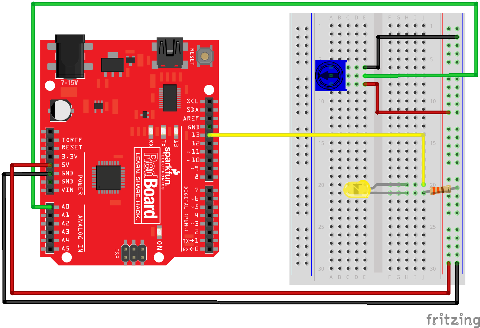
Hardware Hookup
Hook up a potentiometer upward to an Arduino based on the diagram below.
Arduino Code
Later on the footling blue potentiometer is hooked upward, Upload the following code on the Arduino. This code reads the potentiometer value and sends the measured value over the serial line.
// potentiometer.ino // reads a potentiometer and sends value over series int sensorPin = A0; // The potentiometer is continued to analog pin 0 int ledPin = 13; // The LED is connected to digital pivot 13 int sensorValue; // an integer variable to store the potentiometer reading void setup() // this part runs once when the sketch starts { // brand the LED pin (pin thirteen) an output pin pinMode(ledPin, OUTPUT); // initialize serial advice at 9600 baud Series.begin(9600); } void loop() // this function runs repeatedly after setup() finishes { sensorValue = analogRead(sensorPin); // read the voltage at pivot A0 Serial.println(sensorValue); // Output voltage value to Serial Monitor if (sensorValue < 500) { // if sensor output is less than 500, digitalWrite(ledPin, LOW); } // Plow the LED off else { // if sensor output is greater than 500 digitalWrite(ledPin, Loftier); } // Keep the LED on filibuster(100); // Suspension 100 milliseconds before next reading } Python Lawmaking
The PySerial library needs to exist installed earlier nosotros can use PySerial to read the sensor data the Arduino spits out over the series line. Install PySerial with the command below. Make sure you activated the (live_plot) virtual surround when the install command is entered.
(live_plot)> conda install -y pyserial or
(venv)$ pip install pyserial At the top of the Python script, nosotros import the necessary libraries:
# live_plot_sensor.py import time import serial import matplotlib.pyplot equally plt import matplotlib.animation as animation Next, we need to build an animate() function like we did above when we build our live plot from a data file and our live plot from a web API.
# animation function def animate ( i , data_lst , ser ): # ser is the serial object b = ser . readline () string_n = b . decode () string = string_n . rstrip () flt = float ( string ) data_lst . append ( flt ) # Add x and y to lists data_lst . append ( flt ) # Limit the information listing to 100 values data_lst = data_lst [ - 100 :] # clear the final frame and draw the adjacent frame ax . clear () ax . plot ( data_lst ) # Format plot ax . set_ylim ([ 0 , 1050 ]) ax . set_title ( 'Potentiometer Reading Live Plot' ) ax . set_ylabel ( 'Potentiometer Reading' ) Now we demand to create our data_lst, fig and ax objects, as well as instantiate the serial object ser. Notation that the COM# will may exist dissimilar for you based on which COM port the Arduino is continued to. On MacOS or Linux, the com port will be something like /dev/ttyUSB0 instead of COM7. If you are using MacOS or Linux, y'all may need to alter the permissions of the com port earlier the script volition run. The command sudo chown root:peter /dev/ttyUSB0 changes the group corresponding to ttyUSB0 to peter. You volition accept to modify this command based on your MacOS or Linux username and port number.
# create empty listing to store information # create figure and axes objects data_lst = [] fig , ax = plt . subplots () # ready upward the serial line ser = serial . Serial ( 'COM7' , 9600 ) # change COM# if necessary time . slumber ( 2 ) print ( ser . proper name ) Then we demand to call our animation using Matplotlib'southward FuncAnimate grade. After the animation is finished, we should close the serial line
# run the animation and testify the effigy ani = blitheness . FuncAnimation ( fig , animate , frames = 100 , fargs = ( data_lst , ser ), interval = 200 ) plt . show () # afterward the window is airtight, close the serial line ser . close () print ( "Serial line closed" ) The unabridged Python script is below:
# live_plot_sensor.py import time import series import matplotlib.pyplot as plt import matplotlib.animation every bit animation # animation office def animate ( i , data_lst , ser ): # ser is the serial object b = ser . readline () string_n = b . decode () string = string_n . rstrip () try : flt = float ( cord ) data_lst . append ( flt ) data_lst . append ( flt ) except : laissez passer # Add x and y to lists # Limit the data list to 100 values data_lst = data_lst [ - 100 :] # clear the last frame and draw the side by side frame ax . clear () ax . plot ( data_lst ) # Format plot ax . set_ylim ([ 0 , 1050 ]) ax . set_title ( "Potentiometer Reading Alive Plot" ) ax . set_ylabel ( "Potentiometer Reading" ) # create empty list to store data # create figure and axes objects data_lst = [] fig , ax = plt . subplots () # set up the serial line ser = serial . Serial ( "/dev/ttyUSB0" , 9600 ) # change COM# if necessary time . sleep ( two ) print ( ser . name ) # run the animation and prove the effigy ani = blitheness . FuncAnimation ( fig , animate , frames = 100 , fargs = ( data_lst , ser ), interval = 100 ) plt . show () # after the window is airtight, close the serial line ser . close () print ( "Serial line closed" ) Run the script using the Anaconda Prompt or a last:
(live_plot)> python live_plot_sensor.py Twist the trivial bluish potentiometer while the script is running and watch the blithe line on the plot update.
Summary
In this post, nosotros created a couple of live auto-updating animated line plots with Matplotlib. The fundamental to building blithe plots with Matplotlib is to define the plot in an blitheness office and and so call your animation function with Matplotlib's FuncAnimation course.
Support
What to learn about building other types of plots with Matplotlib? Check out my volume Problem Solving with Python on Amazon (Affiliate Link):


Source: https://pythonforundergradengineers.com/live-plotting-with-matplotlib.html
Posted by: sosacolusay.blogspot.com
0 Response to "How To Draw Q-q Plot Using Python"
Post a Comment